Designing the next plate
We ran a case study to measure how six acquisition rules compare when choosing which 96 protein variants to assay next, as a retrospective benchmark on a fully measured fitness landscape of protein GB1, in which four amino acids vary. Rules that target high predicted fitness recover more than three times as much of the top tier as making analogues of the best variant so far, the standard bench practice, and more than twenty times as much as uniform sampling.
Motivation
This case study is about using active learning for optimal experiment design. This framework is versatile and applies to many problems that scientists face: how to optimise a molecular formula to reach a given property in the design of a material, and specifically which molecules to test next. In our case, we focused on the optimisation of a protein variant on a predefined fitness assay.
The assay and the task themselves might not be relevant for a real application. We specifically chose this dataset because the fitness landscape was almost fully determined, and therefore it allowed us to run a retrospective benchmark of the methods. Without such a dataset, we would have needed to run wet lab experiments, which we do not have the capacity for. Moreover, we like the fact that this dataset relies on a biological assay and was designed to assess epistatic effects.
Our motivation is threefold. We aim to show the techniques of active learning to scientists who are potentially unaware of them. We also aim to gain hands-on expertise and to demonstrate our ability to run a rigorous benchmark and a small research piece. Finally, we simply enjoy solving problems, and we are committed to producing public and reproducible artifacts of the best quality.
Background
A protein of length L has 20L possible sequences. Even restricted to four positions, as here, there are 160,000 variants, and a laboratory measures them a plate at a time. Plates are usually 96-well, hence biologists collect assay values 96 by 96. The practical question is which 96 to measure next, given the already collected measurements.
Active learning is a solution to this kind of problem. The cost of exhaustive biological measurements is replaced by an ad hoc prediction of expected fitness and of the uncertainty about these predictions. Each round, a surrogate model is fitted to the measurements in hand, an acquisition rule scores the untested candidates, finally the highest-scoring batch is measured, and its labels are added to our running dataset. The acquisition rule is the component compared in this case study. It maps the surrogate’s predictions and uncertainties onto a choice of batch.
We performed the evaluation retrospectively. The landscape was downloaded from the FLIP benchmark export, hence all the variants we consider have already been measured. We proceed in hiding the labels, revealing them when the acquisition rule decides the next batch. It allows us to remove assay noise and cost from the comparison while leaving the decision problem intact.
Protein
Protein G domain B1 (GB1) is a 56-residue domain from streptococcal protein G that binds the constant region of immunoglobulin G. It folds without cofactors, and its structure has been resolved since 1993.
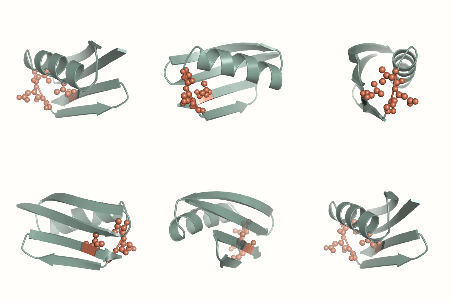
Wu and colleagues selected the four positions because they carry the strongest interactions in the domain: the sites contain 12 of the top 20 positively epistatic interactions among all pairwise interactions in protein GB1, as measured in their earlier survey of single and double mutants. Epistasis means the effect of one mutation depends on which others are present: single residue variants with lower fitness can hinder the path to a two residue variant with higher fitness than the starting point.
The four residues are neighbours in space where they are distant in sequence, clustered around the β3 and β4 strands. Mutating them together alters one small packed region.
Measurement
Wu and colleagues built an exhaustive library of measurements by mutating the four codons. They then measured the fitness of all the variants at once by mRNA display coupled to Illumina sequencing. With that method, each protein variant is physically attached to the messenger RNA that encodes it. These complexes are then mixed with immunoglobulin G, the target of the protein, and recording which proteins are effectively bound to the immunoglobulin G enriches the sequences of the variants that bind more strongly. This enrichment can be read by counting reads: the mRNAs enable this counting, acting like barcodes that identify the protein version.
Fitness in this assay is the enrichment, normalised to the wild type. For variant i, the value of the fitness is the ratio of its read count after selection to before, divided by the same ratio for the wild type. The wild-type sequence V39D40G41V54 therefore has fitness 1 by construction, and a variant at fitness 4 was enriched four times as strongly.
Variants with fewer than ten reads before selection were discarded, which leaves 149,361 of the 160,000 possible sequences. And because fitness is a ratio of counts, its precision depends on those counts: a variant near the ten-read floor carries substantial sampling error, therefore the exact membership of the top of the ranking is partly a property of sequencing depth. The authors report a correlation of 0.97 between this dataset and their earlier measurements of the same mutants, so the bulk of the signal is reproducible.
The remaining 6.6 per cent of sequences were imputed by regression in the original paper. We didn’t use these.
Library
We restricted our pool to variants within three mutations of the wild type for tractability reasons. Our dataset is composed of 28,187 variants, 19% of the measured landscape.
FWAA.This subsampling puts 64% of the landscape’s true top 1% out of reach, including the global optimum, which is a quadruple mutant. The best a campaign can possibly find in our pool is a variant of 6.275 fitness.
Within the pool, we globally define the target as the 99th percentile of fitness, 2.8539, and we refer to recovery as the discovery of the 282 variants above it.
Procedure
We start a campaign from the wild type plus twelve of its single mutants, drawn at random for each replicate. That is, we start with 13 measurements in hand before the first acquisition.
In this study, we did not vary the surrogate. We chose a Gaussian process with a squared-exponential kernel over one-hot encoded sequence. On one-hot features, squared Euclidean distance is twice the Hamming distance, hence the kernel is a smooth measure of sequence similarity. It is refit from scratch every round on the revealed labels only, with its hyperparameters set by marginal likelihood. A Gaussian process is used because it returns a distribution rather than precise numbers. Predictions are linked with uncertainty, and actually four of the six acquisition rules we test need that uncertainty to function.
Each round, we collect new labels for 96 chosen variants. 96 because biologists usually run assays with 96-well plates. The total budget is 96 variants per round for 8 rounds, so 781 assays in total, or 3% of the pool. The six rules are evaluated on 24 random seeds, that are the same across rules, hence the comparisons between the rules are paired: same starting measurements, same budget, same landscape.
Each acquisition rule exhaustively scores the 28,187 untested variants per round. It is common to pre-filter the pool to make the expensive rules affordable. But doing so gives the rules unequal search spaces and confounds the comparison, so we did not rely on a shortlist here.
Because we assay variants batch by batch and not variant by variant, a relevant acquisition rule might use this to its advantage. Indeed, assaying in one batch 96 close variants, even if the prediction for each one is uncertain but potentially highly rewarding, is in general not optimal. A strategic choice is to ensure diversity in the next round, so as not to spend multiple measurements on correlated values.
Acquisition
qLogNEI rewards expected improvement. It scores a whole plate by how much it expects the best measurement in that plate to exceed the best already in hand, averaged over the surrogate's posterior. A variant scores well either because it is predicted to be good or because it might be, so uncertainty is rewarded when it could pay.
GIBBON, also known as max-value entropy search, chooses the plate that most reduces the surrogate's uncertainty about the value of the optimum, rather than the plate most likely to contain it. It actively searches information about the location of the peak, but not necessarily the peak itself.
Greedy takes the 96 variants with the highest predicted fitness. No notion of uncertainty and no notion of a plate acquisition. It ranks candidates one by one and takes the top 96 of the list.
Uncertainty is our baseline that takes the 96 variants the surrogate is the least sure about. It is a very common active learning heuristic, aimed at reducing error everywhere rather than finding the optimum.
SAR is an expert heuristic we defined as “Assay things that look like the winner”. It takes 96 variants closest in sequence to the best measured so far, which is how a bench campaign is usually run and needs no model at all.
Random finally is a uniform draw from the untested pool. It is our null baseline and reference.
The two Bayesian rules build a plate by choosing one variant at a time and conditioning on having chosen it. This mechanism ensures diversity because the second pick is scored knowing the first is already assayed. The three baselines have no such mechanism, that is they rank candidates individually and take the top of the list.
Round
We present the expected improvement campaign on seed 18.
- assayed so far
- 589
- in the top 1%
- 30 of 96
- best in hand
- 6.124
- rank correlation
- 0.580
- predicted uncertainty
- 0.59 to 1.39
The 32 most confident picks at round 6 returned 18 variants above the target, topping out at 5.772, and accounted for most of the round’s yield. The 32 least confident picks returned only 3 above the target. But one of them was VWAA, which the model predicted at 1.873 give or take 1.214, and which was measured 6.124. The model was wrong by more than a factor of three, and it was the best variant the campaign had seen: the running best rose from 5.495 to 6.124 on that measurement.
VWAA was not selected on its predicted value, which was unremarkable, but on its uncertainty. Expected improvement scores a candidate by the size of the gain it could produce, weighted by how likely that gain is, and a wide posterior admits a large gain. Most such picks returned nothing. This one advanced the campaign further than the 32 confident picks combined.
Results
| Rule | Top 1% recovered | 95% interval | Best fitness | Enrichment |
|---|---|---|---|---|
| qLogNEI | 66% | 63% to 70% | 6.03 | 24.0× |
| Greedy | 63% | 61% to 65% | 5.84 | 22.6× |
| SAR | 20% | 19% to 22% | 5.75 | 7.2× |
| GIBBON | 8% | 7% to 11% | 5.67 | 3.0× |
| Uncertainty | 3% | 2% to 4% | 4.59 | 1.1× |
| Random | 3% | 3% to 3% | 4.81 | 1.0× |
Recovery is defined as the fraction of the pool’s 282 best variants that a campaign has measured by the end. Intervals are bias-corrected bootstrap over 24 replicates. Enrichment is recovery relative to what uniform sampling of the same budget returns.
Four of the five rules are ahead of the reference, each at a Holm-adjusted p below 0.001. Expected improvement recovers 66% of the top tier and greedy exploitation 63%, both roughly 24 times what uniform sampling returns at the same budget. Making analogues of the current winner reaches 20%. Max-value entropy search reaches 8%, ahead of random but by a factor of three.
The performance of uncertainty sampling is indistinguishable from random sampling: a paired difference of 0.001 with an interval from -0.008 to 0.008.
The two leading rules are not separated by this experiment. Paired over all 24 replicates, expected improvement is ahead of greedy by 0.039, with a bootstrap interval of 0.000 to 0.076 and a signed-rank p of 0.089. The interval excludes zero; the rank test does not reach significance.
Extrapolation
At the end of the campaigns, we refit the surrogate on that campaign’s measurements and ask it a question that it was not trained for: rank all 149,361 variants of the full landscape, including the 121,174 quadruple mutants, for now unexplored.
| Rule | Rank given to the global optimum | Top ten in | Best variant it would propose | Quadruple mutants proposed |
|---|---|---|---|---|
| qLogNEI | 2 | 19 of 24 | 8.67 | 88 of 96 |
| Greedy | 151 | 6 of 24 | 8.37 | 68 of 96 |
| SAR | 265 | 0 of 24 | 5.50 | 2 of 96 |
| GIBBON | 641 | 3 of 24 | 7.05 | 26 of 96 |
| Uncertainty | 1,281 | 0 of 24 | 6.19 | 34 of 96 |
| Random | 1,503 | 0 of 24 | 6.16 | 23 of 96 |
The rank we describe in the table is the median position the campaign’s final model gives to FWAA, the fittest variant measured (8.762), which is a four-position mutant.
The expected improvement model places the global optimum at median rank 2 out of 148,600 across its seeds, and inside its top ten in 19 of 24 campaigns. A model that never measured quadruples identifies the best quadruple mutant in the landscape. Its 96 proposals average Hamming distance 3.9.
Analogue-making ends with the highest hit rate of all the rules: 81of its 96 proposals fall in the full landscape’s top 1%, more than the expected improvement acquisition rule (68).
Interpretation
In this experiment, pointing the model at the optimum is what matters. The acquisition rules that were targeted toward sampling the maximum fitness beat uniform sampling by a factor of twenty. An hypothesis is that the performance of the simplistic greedy acquisition rule is explained by a lack of complexity or vastitude of the dataset.
Sophistication was not required to collect the best samples. Expected improvement and plain argmax of the posterior mean are not separated by this task. If the goal is to harvest the top of a landscape within a fixed budget, a surrogate that fits it and simple exploitation captured essentially all of the available gain here.
Sophistication was required to extrapolate. The two rules are however sharply separated by how their models extrapolate correctly about sequences they have not yet visited.
The scope is narrow: four coupled positions, a surrogate that fits this landscape, and a budget of a few per cent of the library. The ranking of the rules and the size of the gap over random are yet what we expect transferable parts.
Limitations
The oracle is a lookup and we did not intend to model assay noise in this task. Though, in a real wetlab setting, batches come with a nuisance called batch effects, and measurements across different batches are not directly comparable: they can be monotonically shifted, in the best case.
Fitness is estimated from read counts, hence recovering the true top 1% is in part recovering measurement error.
The pool is fixed and finite. In a real setting, a programme designs variants rather than selecting from an enumerated list, and synthesisability constrains the compounds that can be proposed.
Reproduction
The 144 campaigns ran across 24 machines, one seed per machine, on Intel(R) Core(TM) i7-14700K processors. A campaign is determined by its seed together with the arithmetic thread count, since floating-point summation is not associative and reorders near-ties among tens of thousands of candidates.
The primary endpoint, the reference rule, the interval method and the multiplicity correction are set in the configuration file. The metrics in section 10 are secondary and were added once the primary result was known.
| Rule | Seconds per campaign | Share of the total |
|---|---|---|
| GIBBON | 14,320 | 64.5% |
| qLogNEI | 7,791 | 35.1% |
| Greedy | 51 | 0.2% |
| Uncertainty | 50 | 0.2% |
| SAR | <1 | <0.1% |
| Random | <1 | <0.1% |
The whole benchmark cost 148 core-hours, of which the two Bayesian rules account for 99.5%, because they score 28,187 candidates once per variant chosen rather than once per plate. Because an hour of processor time is not what limits a campaign whose measurements take multiple weeks, wall clock was not compared in this study.
Repositorygithub.com/Sagace-Labs/gb1-active-learningThe code, the run records and the report. MIT.
- summary.csvRecovery, intervals and enrichment per rule
- comparisons.csvPaired differences against the reference
- head_to_head.csvThe two leading rules
- secondary.csvArea under the curve, regret, recommendation lift
- extrapolation.csvEach final model scored on the full landscape
- curves.csvEvery round of every campaign
- provenance.jsonPool and configuration hashes, machines, versions
References
- Wu N. C., Dai L., Olson C. A., Lloyd-Smith J. O., Sun R. (2016). Adaptation in protein fitness landscapes is facilitated by indirect paths. eLife 5.doi.org/10.7554/eLife.16965All fitness values come from this study. It selects the four positions and describes the assay.
- doi.org/10.1016/j.cub.2014.09.072This survey measures pairwise epistasis in GB1. We selected the four positions from its results.
- Dallago C., Mou J., Johnston K. E., Wittmann B. J., Bhattacharya N., Goldman S. et al. (2021). FLIP: Benchmark tasks in fitness landscape inference for proteins.doi.org/10.1101/2021.11.09.467890We downloaded the landscape from this benchmark.
- Gallagher T., Alexander P., Bryan P., Gilliland G. L. (1994). Two Crystal Structures of the B1 Immunoglobulin-Binding Domain of Streptococcal Protein G and Comparison with NMR. Biochemistry 33 4721-4729.doi.org/10.1021/bi00181a032The structure figure shows these coordinates.
- Ament S., Daulton S., Eriksson D., Balandat M., Bakshy E. (2023). Unexpected Improvements to Expected Improvement for Bayesian Optimization. arXiv.doi.org/10.48550/arXiv.2310.20708The qLogNEI rule uses this acquisition function.
- Moss H. B., Leslie D. S., Gonzalez J., Rayson P. (2021). GIBBON: General-purpose Information-Based Bayesian OptimisatioN. arXiv.doi.org/10.48550/arXiv.2102.03324This paper defines max-value entropy search. We call the rule GIBBON.
- Balandat M., Karrer B., Jiang D. R., Daulton S., Letham B., Wilson A. G. et al. (2019). BoTorch: A Framework for Efficient Monte-Carlo Bayesian Optimization. arXiv.doi.org/10.48550/arXiv.1910.06403We use this library for the acquisition functions and the batch construction.
- Graff D. E., Shakhnovich E. I., Coley C. W. (2021). Accelerating high-throughput virtual screening through molecular pool-based active learning. Chemical Science 12 7866-7881.doi.org/10.1039/D0SC06805EOur benchmark follows the pool-based design in this work.
We are an open research lab.
For research use only. Retrospective benchmark on a public dataset.